# Import necessary libraries for optical neural network simulation
import torch
from torch import nn
import svetlanna as sv

# Import units for physical measurements
from svetlanna.units import ureg

# Import wavefront and optical setup classes
from svetlanna import Wavefront
from svetlanna import LinearOpticalSetup

# Import MNIST dataset and data transformation utilities
from torchvision.datasets import MNIST
import torchvision.transforms as transforms
from svetlanna.transforms import ToWavefront

# Import visualization tools
import matplotlib.pyplot as plt
from svetlanna.visualization import show_stepwise_forward, show_structure, show_specs
Optical Neural Network
1. Simulation parameters
In this example notebook, we will implement a simple architecture of an optical neural network based on the article [1] :
In general, the phase and amplitude of each neuron can be learnable parameters, providing a complex-valued modulation at each layer, which improves the inference performance of the diffractive network.
… we first trained it as a digit classifier to perform automated classification of handwritten digits, from to . For this task, phase-only transmission masks were designed by training a five-layer with images ( validation images) from the MNIST handwritten digit database.
We then used continuous-wave illumination at …
Some information from the supplementary material (regarding MNIST classification):
Because we consider coherent illumination, the input information can be encoded in the amplitude and/or phase channels of the input plane.
For each layer of the , we set the neuron size to be …
At the detector/output plane, we measured the intensity of the network output…
In another article [2] by the same authors, some details were clarified:
In our numerical simulations, we used a neuron size of approximately
In addition, the height and width of each diffractive layer was set to include neurons per layer.
# Calculate the wavelength from the frequency
c = 299_792_458 * (ureg.m / ureg.s)  # Speed of light
wavelength = c / (400 * ureg.GHz)  # Wavelength at 0.4 THz [m]
print(f"lambda: {wavelength / ureg.um:.3f} um")

# Calculate neuron size based on wavelength (from the article)
neuron_size = 0.53 * wavelength  # [m]
print(f"Neuron size: {neuron_size / ureg.um:.3f} um")

# Define the physical size of each diffractive layer
# The article specifies (8 x 8) [cm] and 200 x 200 neurons
Nx, Ny = 200, 200  # Number of neurons in each dimension
W = Nx * neuron_size  # Width [m]
H = Ny * neuron_size  # Height [m]

print(f"Layer size: {W / ureg.cm:.3f} cm x {H / ureg.cm:.3f} cm")
Output:
lambda: 749.481 um
Neuron size: 397.225 um
Layer size: 7.945 cm x 7.945 cm
# Create simulation parameters for the optical system
# These parameters define the spatial grid and wavelength for all simulations
SIM_PARAMS = sv.SimulationParameters(
{
"W": torch.linspace(-W / 2, W / 2, Nx), # Width axis
"H": torch.linspace(-H / 2, H / 2, Ny), # Height axis
"wavelength": wavelength, # Operating wavelength
}
)2. Dataset preparation
In this example MNIST Dataset is used. From [2] :
Input objects were encoded in the amplitude channel (MNIST) of the input plane and were illuminated with a uniform plane wave at a wavelength of to match the conditions introduced in [1] for all-optical classification.
So, we need to perform amplitude modulation of each image from the dataset.
# Define transformation pipeline for MNIST images
# 1. Convert to tensor
# 2. Resize to 100x100 pixels (using nearest neighbor interpolation)
# 3. Pad to 200x200 to match the diffractive layer size
# 4. Convert to wavefront with amplitude modulation
to_wavefront_transform = transforms.Compose(
    [
        transforms.ToTensor(),
        transforms.Resize(
            size=(100, 100),
            interpolation=transforms.InterpolationMode.NEAREST,
        ),
        transforms.Pad(
            padding=(50, 50, 50, 50),  # Pad equally on all sides
            fill=0,  # Fill with zeros (no light)
        ),
        ToWavefront(modulation_type="amp"),  # Encode in amplitude channel
    ]
)


# Load MNIST training dataset
training_data = MNIST(
    root="data",
    train=True,
    download=True,
    transform=to_wavefront_transform,
)

# Load MNIST test dataset
test_data = MNIST(
    root="data",
    train=False,
    download=True,
    transform=to_wavefront_transform,
)

print(f"Train data size: {len(training_data)}")
print(f"Test data size : {len(test_data)}")
Output:
Train data size: 60000
Test data size : 10000
# Visualize some examples from the training dataset
n_examples = 4
torch.random.manual_seed(78)
train_examples_ids = torch.randperm(len(training_data))[:n_examples]
fig, axs = plt.subplots(2, n_examples)
for ind_ex, ind_train in enumerate(train_examples_ids):
wavefront, wf_label = training_data[ind_train]
# Show intensity (|E|^2)
plt.subplot(2, n_examples, ind_ex + 1)
plt.title("$|E|^2$")
plt.imshow(wavefront.intensity, cmap="hot")
# Show phase (arg(E))
plt.subplot(2, n_examples, ind_ex + 1 + n_examples)
plt.title("arg($E$)")
plt.imshow(wavefront.angle(), cmap="twilight_shifted")
plt.show()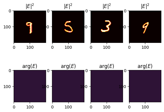
3. Optical Network
Information from the supplementary material of [1] for MNIST classification:
Following the corresponding design, the axial distance between two successive 3D-printed layers was set to be cm…
The distance between the detector/output plane and the last layer of the optical neural network was adjusted as cm…
From [2] :
… the axial distance between the successive diffractive layers is set to be as in [1] …
See Figure 2A from [1] . See Figure 1(a) from [2] .
Detector
… size of these detectors …
In [2] , the authors propose using CrossEntropyLoss. For this purpose, the following values were calculated for each output:
… the measured intensities by D detectors at the output plane are normalized such that they lie in the interval for each sample. With denoting the total optical signal impinging onto the detector at the output plane, the normalized intensities, , can be found by,
# Create detector segments for each digit class (0-9)
# Each detector has size 6.4λ × 6.4λ as specified in the article

def create_segment_mask(x: int, y: int):
    """Create a detector mask at specified position (x, y)."""
    dx = dy = int(6.4 * wavelength / neuron_size)

    res = torch.zeros((Nx, Ny))
    res[
        (Ny - dy) // 2 + y : (Ny + dy) // 2 + y, (Nx - dx) // 2 + x : (Nx + dx) // 2 + x
    ] = 1.0
    return res


d = int(6.4 * wavelength / neuron_size)

# Create 10 detector masks arranged in a specific pattern
# (matching the detector layout from the article)
detector_segment_masks = torch.stack(
    [
        create_segment_mask(-int(2.7 * d), -int(2.7 * d)),  # Detector for digit 0
        create_segment_mask(0, -int(2.7 * d)),              # Detector for digit 1
        create_segment_mask(int(2.7 * d), -int(2.7 * d)),   # Detector for digit 2
        create_segment_mask(-int(3 * d), 0),                # Detector for digit 3
        create_segment_mask(-int(1 * d), 0),                # Detector for digit 4
        create_segment_mask(int(1 * d), 0),                 # Detector for digit 5
        create_segment_mask(int(3 * d), 0),                 # Detector for digit 6
        create_segment_mask(-int(2.7 * d), int(2.7 * d)),   # Detector for digit 7
        create_segment_mask(0, int(2.7 * d)),               # Detector for digit 8
        create_segment_mask(int(2.7 * d), int(2.7 * d)),    # Detector for digit 9
    ],
    dim=-1,
)


# Visualize the detector layout
plt.figure(figsize=(10, 4))
for i in range(10):
    plt.subplot(2, 5, i + 1)
    plt.imshow(
        detector_segment_masks[..., i] + torch.sum(detector_segment_masks, axis=-1),
        cmap="gray",
    )
    plt.title(f"Class {i}")
    plt.gca().set_axis_off()
plt.show()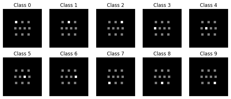
Network
class Model(nn.Module):
    """
    Diffractive Deep Neural Network (D²NN) for MNIST classification.

    The architecture consists of:
    - 5 diffractive layers with phase-only modulation
    - Free-space propagation between layers (40λ distance)
    - Final propagation to detector plane
    - 10 detectors for digit classification
    """

    def __init__(self):
        super().__init__()

        elements = []

        # Create 5 diffractive layers with free-space propagation
        for _ in range(5):
            # Free-space propagation using Angular Spectrum method
            elements.append(
                sv.elements.FreeSpace(
                    simulation_parameters=SIM_PARAMS,
                    distance=40 * wavelength,  # Distance between layers: 40λ
                    method="AS",  # Angular Spectrum propagation
                )
            )
            # Diffractive layer with trainable phase mask
            elements.append(
                sv.elements.DiffractiveLayer(
                    simulation_parameters=SIM_PARAMS,
                    mask=sv.ConstrainedParameter(
                        torch.full((Nx, Ny), torch.pi),  # Initialize with π
                        min_value=0,
                        max_value=2 * torch.pi,  # Phase-only: [0, 2π]
                    ),
                )
            )

        # Final propagation to detector plane
        elements.append(
            sv.elements.FreeSpace(
                simulation_parameters=SIM_PARAMS,
                distance=40 * wavelength,
                method="AS",
            )
        )

        self.setup = LinearOpticalSetup(elements)

    def forward(self, wavefront: Wavefront):
        # Propagate through the optical setup
        wavefront = self.setup(wavefront)
        intensity = wavefront.intensity

        # Calculate total intensity at each detector
        I_l = (intensity[..., None] * detector_segment_masks).sum(dim=(-2, -3))

        # Normalize intensities to [0, 10] range (as in the article)
        I_l_norm = I_l / torch.max(I_l, dim=-1, keepdim=True).values * 10
        return I_l_norm
# Instantiate the optical neural network model
model = Model()Example of wavefront propagation
# Select an example wavefront from the training data
example_wf = training_data[128][0]
# Visualize the structure of the optical setup
show_structure(model.setup)─→┨ ┠─→
─→▒▒─→
─→┨ ┠─→
─→▒▒─→
─→┨ ┠─→
─→▒▒─→
─→┨ ┠─→
─→▒▒─→
─→┨ ┠─→
─→▒▒─→
─→┨ ┠─→
# Display specifications of each element in the optical setup
show_specs(model.setup)
<svetlanna.visualization.widgets.SpecsWidget object at 0x132d6a310># Show step-by-step propagation through the optical network
show_stepwise_forward(model.setup, input=example_wf, simulation_parameters=SIM_PARAMS)<svetlanna.visualization.widgets.StepwiseForwardWidget object at 0x103a00350>4. Training the Network
4.1. Training preparation
DataLoaders
Information from the supplementary material of [1] for MNIST classification:
The training batch size was set to be …
For this task, phase-only transmission masks were designed by training a five-layer with images ( validation images) from the MNIST (Modified National Institute of Standards and Technology) handwritten digit database.
We will use training dataset for training and test dataset for testing, provided with torchvision.datasets.MNIST.
We will use batch size of 128 to speed up the training process.
# Create data loaders for training and testing
batch_size = 128

train_dataloader = torch.utils.data.DataLoader(
    training_data,
    batch_size=batch_size,
    shuffle=True,  # Shuffle training data
    # num_workers=2,  # Uncomment for parallel data loading
    drop_last=False,
)

test_dataloader = torch.utils.data.DataLoader(
    test_data,
    batch_size=128,
    shuffle=False,  # Don't shuffle test data
    # num_workers=2,  # Uncomment for parallel data loading
    drop_last=False,
)
Optimizer and Loss Function
Information from the supplementary material of [1] for MNIST classification:
We used the stochastic gradient descent algorithm, Adam, to back-propagate the errors and update the layers of the network to minimize the loss function.
Additional information from [2] :
… a back-propagation method by applying the adaptive moment estimation optimizer (Adam) with a learning rate of
We will use the Adam optimizer with a learning rate of 5e-3 to speed up the training process.
# Set up optimizer and loss function
optimizer = torch.optim.Adam(params=model.parameters(), lr=5e-3)
loss_fn = nn.CrossEntropyLoss()
Training and evaluation loops
The training loops are direct copy of those presented at torch documentation .
def train_loop(dataloader, model, loss_fn, optimizer):
    size = len(dataloader.dataset)
    # Set the model to training mode - important for batch normalization and dropout layers
    # Unnecessary in this situation but added for best practices
    model.train()

    for batch, (X, y) in enumerate(dataloader):
        # Compute prediction and loss
        pred = model(X)
        loss = loss_fn(pred, y)

        # Backpropagation
        loss.backward()
        optimizer.step()
        optimizer.zero_grad()

        # Print progress every 100 batches
        if batch % 100 == 0:
            loss, current = loss.item(), batch * batch_size + len(X)
            print(f"loss: {loss:>7f}  [{current:>5d}/{size:>5d}]")


def test_loop(dataloader, model, loss_fn):
    # Set the model to evaluation mode - important for batch normalization and dropout layers
    # Unnecessary in this situation but added for best practices
    model.eval()
    size = len(dataloader.dataset)
    num_batches = len(dataloader)
    test_loss, correct = 0, 0

    # Evaluating the model with torch.no_grad() ensures that no gradients are computed during test mode
    # Also serves to reduce unnecessary gradient computations and memory usage for tensors with requires_grad=True
    with torch.no_grad():
        for X, y in dataloader:
            pred = model(X)
            test_loss += loss_fn(pred, y).item()
            correct += (pred.argmax(1) == y).type(torch.float).sum().item()

    test_loss /= num_batches
    correct /= size
    print(
        f"Test Error: \n Accuracy: {(100 * correct):>0.1f}%, Avg loss: {test_loss:>8f} \n"
    )
    return correct, test_loss
4.2 Training and Evaluating
# Track training progress
test_accuracies = []
test_losses = []

# Evaluate the model before training (random initialization)
accuracy, loss = test_loop(test_dataloader, model, loss_fn)
test_accuracies.append(accuracy)
test_losses.append(loss)

# Train the model for specified number of epochs
epochs = 2
for t in range(epochs):
    print(f"Epoch {t + 1}\n-------------------------------")
    train_loop(train_dataloader, model, loss_fn, optimizer)
    accuracy, loss = test_loop(test_dataloader, model, loss_fn)
    test_accuracies.append(accuracy)
    test_losses.append(loss)

print("Done!")
Output:
Test Error:
 Accuracy: 11.4%, Avg loss: 6.445604

Epoch 1
-------------------------------
loss: 6.450378  [  128/60000]
loss: 0.622412  [12928/60000]
loss: 0.390765  [25728/60000]
loss: 0.244010  [38528/60000]
loss: 0.249918  [51328/60000]
Test Error:
 Accuracy: 94.1%, Avg loss: 0.198886

Epoch 2
-------------------------------
loss: 0.248825  [  128/60000]
loss: 0.252325  [12928/60000]
loss: 0.215309  [25728/60000]
loss: 0.108284  [38528/60000]
loss: 0.154604  [51328/60000]
Test Error:
 Accuracy: 96.2%, Avg loss: 0.136988

Done!
Learning Curves (Cross-Entropy Loss and Accuracy)
# Plot learning curves to visualize training progress
fig, axs = plt.subplots(1, 2, figsize=(10, 3))

# Loss curve
axs[0].plot(range(epochs + 1), test_losses, "-o", label="test")
axs[0].set_ylabel("Loss")
axs[0].set_xlabel("Epoch")
axs[0].legend()

# Accuracy curve
axs[1].plot(range(epochs + 1), test_accuracies, "-o", label="test")
axs[1].set_ylabel("Accuracy")
axs[1].set_xlabel("Epoch")
axs[1].legend()

plt.show()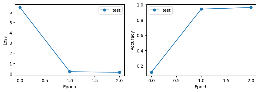
Trained Phase Masks
# Extract and visualize the trained phase masks from all diffractive layers
diffractive_layers = [
    element
    for element in model.setup.elements
    if isinstance(element, sv.elements.DiffractiveLayer)
]

fig, axs = plt.subplots(1, 5, figsize=(15, 4))

for ind_layer, layer in enumerate(diffractive_layers):
    plt.subplot(1, 5, ind_layer + 1)
    trained_mask = layer.mask.detach()

    plt.imshow(trained_mask, cmap="twilight_shifted")
    plt.title(f"DiffractiveLayer {ind_layer + 1}")
plt.show()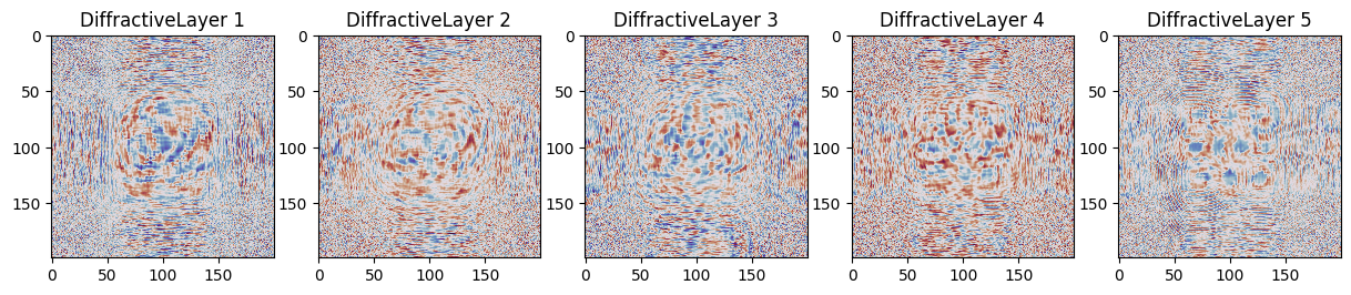
# Display final specifications after training
show_specs(model.setup)
<svetlanna.visualization.widgets.SpecsWidget object at 0x136660c90>5. Example of Classification
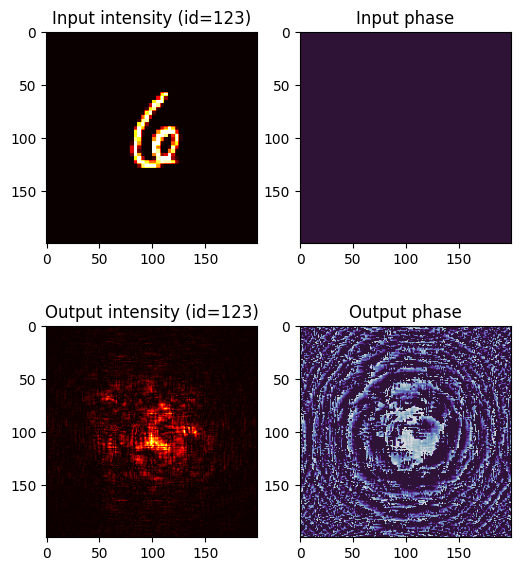
# Select a test sample and visualize the classification process
ind_test = 123
plt.figure(figsize=(6, 7))
test_wavefront, test_target = test_data[ind_test]
# Show input wavefront
plt.subplot(2, 2, 1)
plt.title(f"Input intensity (id={ind_test})")
plt.imshow(test_wavefront.intensity, cmap="hot")
plt.subplot(2, 2, 2)
plt.title("Input phase")
plt.imshow(test_wavefront.angle(), cmap="twilight_shifted", vmin=0, vmax=2 * torch.pi)
# Propagate through the optical network
with torch.no_grad():
test_wavefront_out = model.setup(sv.Wavefront(test_wavefront))
# Show output wavefront
plt.subplot(2, 2, 3)
plt.title(f"Output intensity (id={ind_test})")
plt.imshow(test_wavefront_out.intensity, cmap="hot")
plt.subplot(2, 2, 4)
plt.title("Output phase")
plt.imshow(test_wavefront_out.angle(), cmap="twilight_shifted", vmin=0, vmax=2 * torch.pi)
plt.show()
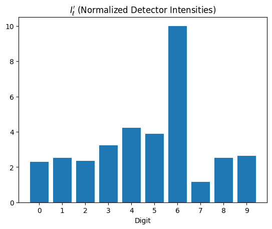
# Display detector responses (classification scores)
with torch.no_grad():
classes = list(range(10))
plt.bar(classes, model(sv.Wavefront(test_wavefront)))
plt.xticks(classes)
plt.xlabel("Digit")
plt.title("$I_\ell'$ (Normalized Detector Intensities)")
plt.show()