Propagation of a Laguerre–Gaussian beam

Laguerre–Gaussian (LG) modes are the natural eigenmodes of a cylindrically symmetric resonator. Every mode with an azimuthal index $l \neq 0$ carries an optical vortex: its phase winds by $2\pi l$ around the axis, the intensity has a dark core, and each photon carries $l\hbar$ of orbital angular momentum.

Wavefront ships with plane_wave, gaussian_beam, spherical_wave and hermite_gauss. LG modes are not built in, so this tutorial shows how to define one on the simulation grid, propagate it with FreeSpace, and verify the result against the analytical solution.

Theory

At a distance $z$ from the waist the $LG_{p,l}$ mode is

E_{p,l}(r, \varphi, z) = \frac{w_0}{w(z)} \left(\frac{\sqrt{2}\,r}{w(z)}\right)^{|l|} L_p^{|l|}\!\left(\frac{2r^2}{w(z)^2}\right) \exp\left(-\frac{r^2}{w(z)^2}\right) e^{i l \varphi}\, e^{i k z}\, e^{i k r^2 / 2R(z)}\, e^{-i \zeta_{p,l}(z)},

with the usual Gaussian-beam quantities

w(z) = w_0\sqrt{1 + (z/z_R)^2}, \quad R(z) = z\left[1 + (z_R/z)^2\right], \quad z_R = \frac{\pi w_0^2}{\lambda},

the generalised Laguerre polynomial $L_p^{|l|}$ , and the Gouy phase

\zeta_{p,l}(z) = (2p + |l| + 1)\arctan(z / z_R).

Two consequences are worth checking numerically:

the beam keeps its shape and only scales with $w(z)$ — LG modes are self-similar;
the bright ring of an $LG_{0,l}$ mode sits at $r = w(z)\sqrt{|l|/2}$ .

Step 1: Defining the mode

Imports and grid


import math
import numpy as np
import torch
import matplotlib.pyplot as plt
 
from svetlanna import SimulationParameters, Wavefront
from svetlanna.elements import FreeSpace
from svetlanna.units import ureg
 
W0 = 0.15 * ureg.mm
LAM = 632.8 * ureg.nm
Z_R = math.pi * W0 ** 2 / LAM        # Rayleigh range
 
params = SimulationParameters.from_ranges(
    x_range=(-1.5 * ureg.mm, 1.5 * ureg.mm), x_points=1024,
    y_range=(-1.5 * ureg.mm, 1.5 * ureg.mm), y_points=1024,
    wavelength=LAM,
)
 
print(f"Rayleigh range: {Z_R * 1e3:.2f} mm")

Output:


Rayleigh range: 111.70 mm

The generalised Laguerre polynomial

A three-term upward recurrence is enough and stays differentiable:


def laguerre(p: int, alpha: int, x: torch.Tensor) -> torch.Tensor:
    """Generalised Laguerre polynomial L_p^alpha(x)."""
    if p == 0:
        return torch.ones_like(x)
    l_prev, l_cur = torch.ones_like(x), 1 + alpha - x
    for n in range(1, p):
        l_prev, l_cur = l_cur, (
            (2 * n + 1 + alpha - x) * l_cur - (n + alpha) * l_prev
        ) / (n + 1)
    return l_cur

The mode itself

SimulationParameters.meshgrid returns the coordinate grids, so the mode is written directly in the formula of the theory section:


def laguerre_gauss(sim, waist_radius, p=0, l=0, distance=0.0):
    """LG_{p,l} mode of a given waist, evaluated at `distance` from the waist."""
    x, y = sim.meshgrid(x_axis="x", y_axis="y")
    wavelength = float(sim.wavelength)
    k = 2 * math.pi / wavelength
    z_r = math.pi * waist_radius ** 2 / wavelength
 
    r2 = x ** 2 + y ** 2
    r = torch.sqrt(r2)
    phi = torch.atan2(y, x)
 
    w = waist_radius * math.sqrt(1 + (distance / z_r) ** 2)
    inv_R = distance / (distance ** 2 + z_r ** 2)      # 1 / R(z), finite at z = 0
    gouy = (2 * p + abs(l) + 1) * math.atan(distance / z_r)
 
    amplitude = (
        waist_radius / w
        * (math.sqrt(2) * r / w) ** abs(l)
        * laguerre(p, abs(l), 2 * r2 / w ** 2)
        * torch.exp(-r2 / w ** 2)
    )
    phase = l * phi + k * distance + k * r2 * inv_R / 2 - gouy
    return Wavefront(amplitude * torch.exp(1j * phase))

Wavefront is a subclass of torch.Tensor, so wrapping a complex tensor is all it takes to obtain a field that every element of the library accepts.

Step 2: The mode gallery


for p, l in [(0, 1), (0, 3), (1, 2)]:
    wf = laguerre_gauss(params, W0, p=p, l=l)
    plt.imshow(wf.intensity.numpy(), cmap="inferno")
    plt.imshow(wf.phase.numpy(), cmap="twilight", vmin=-math.pi, vmax=math.pi)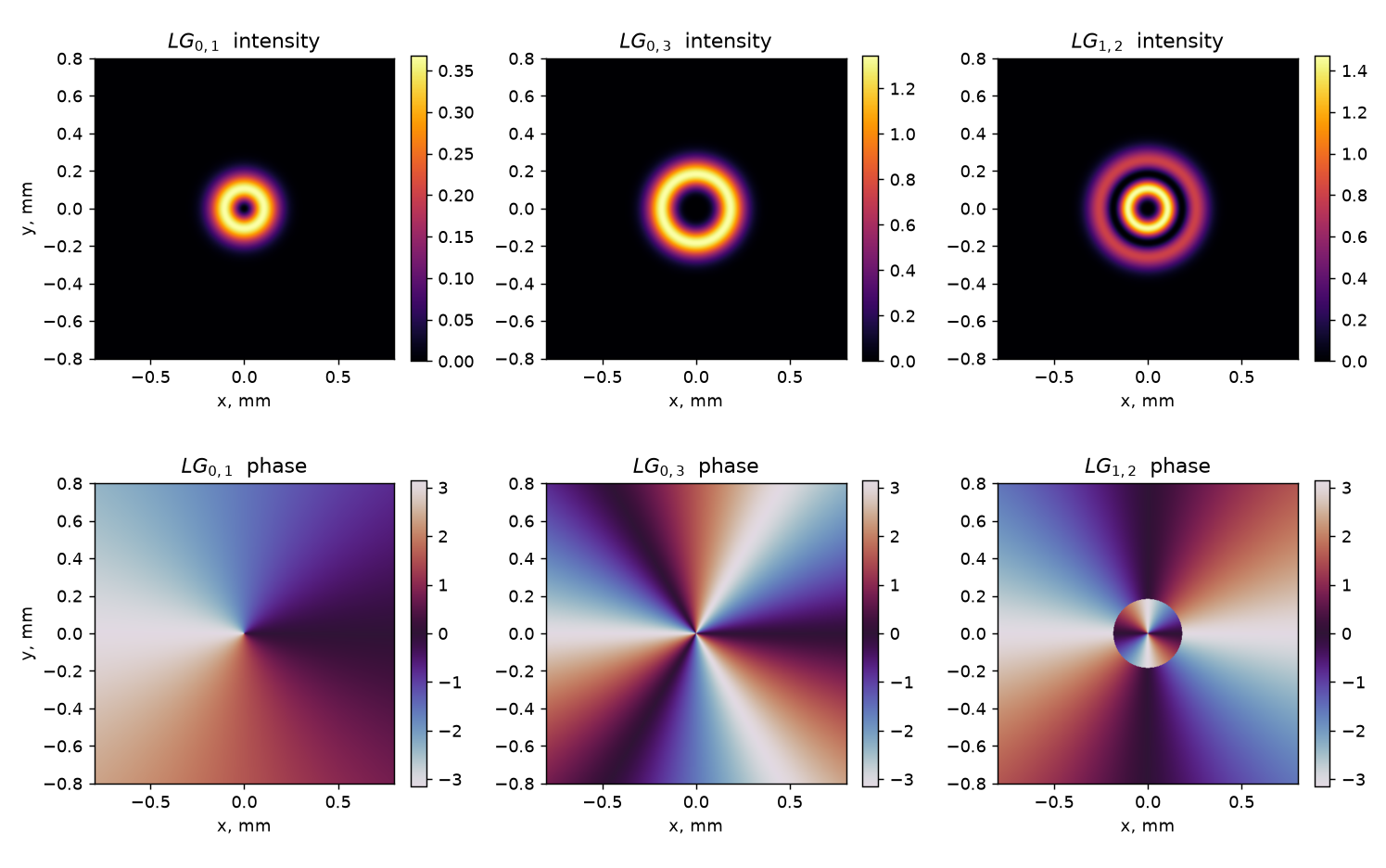

LG mode gallery

The azimuthal index $l$ sets the number of $2\pi$ phase ramps around the axis, and the radial index $p$ adds $p$ dark rings — visible in $LG_{1,2}$ both as a gap in the intensity and as a $\pi$ phase jump across it.

Step 3: Propagation

FreeSpace propagates the field the same way it would any other wavefront:


P, L = 0, 3
wf0 = laguerre_gauss(params, W0, p=P, l=L)
 
for z in [0.5 * Z_R, 1.0 * Z_R, 2.0 * Z_R]:
    numerical = FreeSpace(params, distance=z, method="zpASM")(wf0)
    analytic = laguerre_gauss(params, W0, p=P, l=L, distance=z)
 
    err = (numerical.intensity - analytic.intensity).abs().sum() / analytic.intensity.sum()
    print(f"z = {z * 1e3:7.2f} mm   relative intensity error = {err:.3%}")

Output:


z =   55.85 mm   relative intensity error = 0.250%
z =  111.70 mm   relative intensity error = 0.697%
z =  223.41 mm   relative intensity error = 3.589%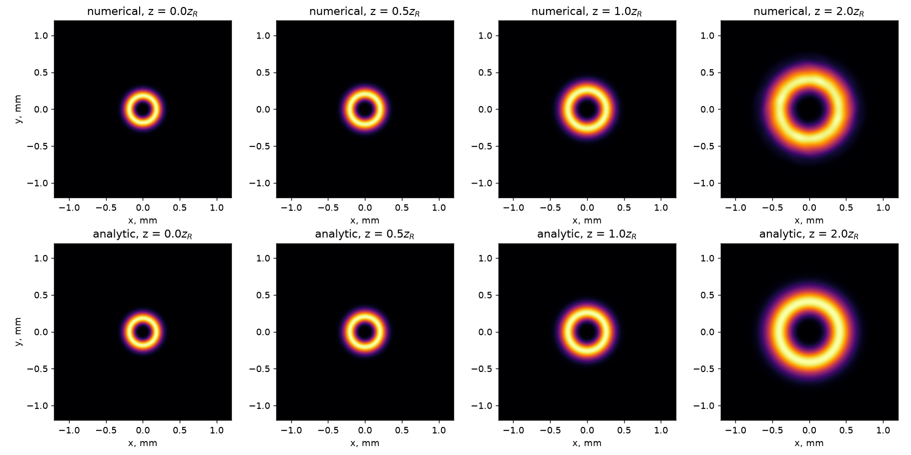

Numerical versus analytic propagation

The numerically propagated field (top row) is indistinguishable from the closed-form solution (bottom row). The error grows with distance because the expanding beam approaches the edge of the computational window — enlarge x_range or increase the padding of the propagator to push it back down.

"zpASM" (zero-padded angular spectrum) avoids the wrap-around artefacts of the plain "ASM" method. For distances of many Rayleigh ranges, prefer "zpRSC".

Step 4: Ring expansion and the vortex charge

Two quantitative checks. First, the radius of the bright ring must follow $w(z)\sqrt{|l|/2}$ :


x = params.x.numpy()
cy = 512   # index of the y = 0 row
 
for z in np.linspace(0, 2 * Z_R, 9):
    wfz = FreeSpace(params, distance=float(z), method="zpASM")(wf0) if z > 0 else wf0
    profile = wfz.intensity.numpy()[cy, cy:]
    radius_numeric = x[cy:][profile.argmax()]
 
    w = W0 * math.sqrt(1 + (z / Z_R) ** 2)
    radius_theory = w * math.sqrt(abs(L) / 2)

Second, interfering the propagated beam with a spherical reference wave turns the phase winding into a visible spiral with exactly $|l|$ arms:


wf_far = FreeSpace(params, distance=2 * Z_R, method="zpASM")(wf0)
reference = Wavefront.spherical_wave(params, distance=-0.6)
 
pattern = (wf_far / wf_far.abs().max() + reference / reference.abs().max()).intensity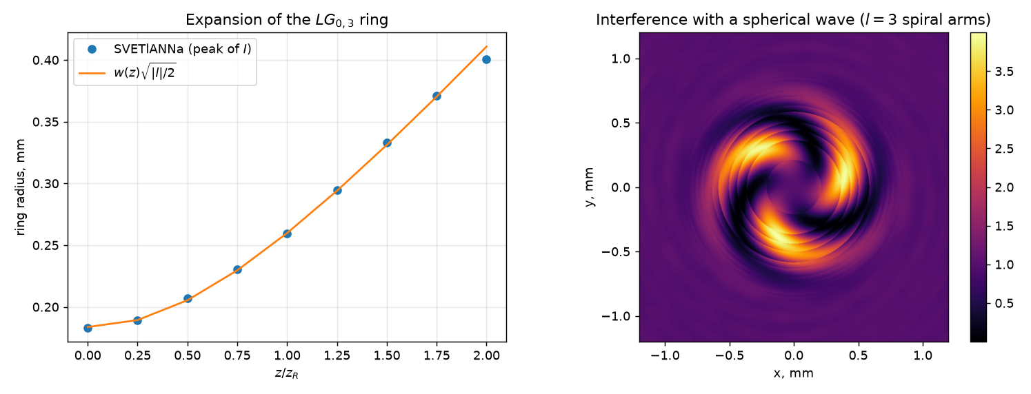

Ring expansion and spiral interference

The measured ring radii lie on the analytical curve, and the interference pattern shows three arms for $l = 3$ — the sign of the topological charge is given by the handedness of the spiral.

Full code


import math
import torch
 
from svetlanna import SimulationParameters, Wavefront
from svetlanna.elements import FreeSpace
from svetlanna.units import ureg
 
W0, LAM = 0.15 * ureg.mm, 632.8 * ureg.nm
Z_R = math.pi * W0 ** 2 / LAM
 
params = SimulationParameters.from_ranges(
    x_range=(-1.5 * ureg.mm, 1.5 * ureg.mm), x_points=1024,
    y_range=(-1.5 * ureg.mm, 1.5 * ureg.mm), y_points=1024,
    wavelength=LAM,
)
 
 
def laguerre(p, alpha, x):
    if p == 0:
        return torch.ones_like(x)
    l_prev, l_cur = torch.ones_like(x), 1 + alpha - x
    for n in range(1, p):
        l_prev, l_cur = l_cur, (
            (2 * n + 1 + alpha - x) * l_cur - (n + alpha) * l_prev
        ) / (n + 1)
    return l_cur
 
 
def laguerre_gauss(sim, waist_radius, p=0, l=0, distance=0.0):
    x, y = sim.meshgrid(x_axis="x", y_axis="y")
    wavelength = float(sim.wavelength)
    k = 2 * math.pi / wavelength
    z_r = math.pi * waist_radius ** 2 / wavelength
 
    r2 = x ** 2 + y ** 2
    w = waist_radius * math.sqrt(1 + (distance / z_r) ** 2)
    inv_R = distance / (distance ** 2 + z_r ** 2)
    gouy = (2 * p + abs(l) + 1) * math.atan(distance / z_r)
 
    amplitude = (
        waist_radius / w
        * (math.sqrt(2) * torch.sqrt(r2) / w) ** abs(l)
        * laguerre(p, abs(l), 2 * r2 / w ** 2)
        * torch.exp(-r2 / w ** 2)
    )
    phase = l * torch.atan2(y, x) + k * distance + k * r2 * inv_R / 2 - gouy
    return Wavefront(amplitude * torch.exp(1j * phase))
 
 
wf0 = laguerre_gauss(params, W0, p=0, l=3)
wfz = FreeSpace(params, distance=Z_R, method="zpASM")(wf0)
 
print("input  max intensity:", float(wf0.max_intensity))
print("output max intensity:", float(wfz.max_intensity))

Things to try

Add a ThinLens and watch the dark core survive focusing — a vortex cannot be focused away.
Superpose $LG_{0,+l}$ and $LG_{0,-l}$ to obtain a petal-shaped mode with $2l$ lobes.
Compare the Gouy phase of $LG_{0,3}$ with that of Wavefront.hermite_gauss(m=3, n=0): modes with the same $2p + |l| = m + n$ share it.
Encode the vortex on a SpatialLightModulator as a fork hologram and recover it in the first diffraction order — see the SLM tutorial.