Diffraction on a sinusoidal phase grating (SLM)

A spatial light modulator (SLM) is a pixelated device that imprints a programmable phase pattern onto a beam. In this tutorial we display a sinusoidal phase grating on a SpatialLightModulator, send a Gaussian beam through it and observe the diffraction orders in the focal plane of a lens. The measured order powers are then compared with the analytical Bessel-function prediction.

Everything on this page runs on the CPU in a few seconds. All figures below were produced by the code shown here.

Theory

A thin phase grating with period $\Lambda$ and peak-to-valley modulation depth $m$ has the transmission function

t(x) = \exp\left[i\,\frac{m}{2}\sin\left(\frac{2\pi x}{\Lambda}\right)\right].

Expanding it in the Jacobi–Anger series gives

t(x) = \sum_{n=-\infty}^{\infty} J_n\!\left(\frac{m}{2}\right) \exp\left(i\,\frac{2\pi n x}{\Lambda}\right),

so the grating splits the beam into discrete diffraction orders. Order $n$ carries the fraction of power

\eta_n = J_n^2\!\left(\frac{m}{2}\right),

where $J_n$ is the Bessel function of the first kind. A lens of focal length $f$ placed behind the grating maps each order onto a spot in its focal plane at

x_n = n\,\frac{\lambda f}{\Lambda}.

Step 1: Simulation grid

Imports and grid


import math
import numpy as np
import torch
import matplotlib.pyplot as plt
 
import svetlanna as sv
from svetlanna import SimulationParameters, Wavefront, LinearOpticalSetup
from svetlanna.elements import SpatialLightModulator, ThinLens, FreeSpace
from svetlanna.elements.slm import QuantizerFromStepFunction, one_step_tanh
from svetlanna.units import ureg
 
params = SimulationParameters.from_ranges(
    x_range=(-2.5 * ureg.mm, 2.5 * ureg.mm), x_points=1024,
    y_range=(-2.5 * ureg.mm, 2.5 * ureg.mm), y_points=1024,
    wavelength=632.8 * ureg.nm,   # HeNe laser
)

The grid step is $\Delta x = 5\ \text{mm} / 1024 \approx 4.9\ \mu\text{m}$ , which comfortably resolves both the SLM pixels and the diffraction orders.

Building the phase mask

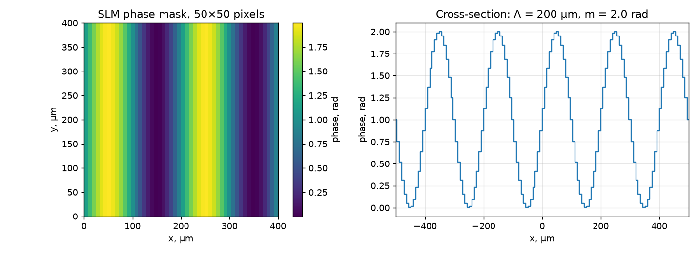
The mask is defined on the SLM pixel grid, not on the simulation grid — the element interpolates it onto the simulation grid automatically. Here the modulator has $400 \times 400$ pixels with an 8 μm pitch, i.e. a 3.2 × 3.2 mm active area.


PITCH  = 8 * ureg.um
NPIX   = 400
PERIOD = 200 * ureg.um    # grating period Λ
DEPTH  = 2.0              # modulation depth m, rad
F      = 150 * ureg.mm    # focal length of the lens
 
px = (torch.arange(NPIX) - (NPIX - 1) / 2) * PITCH
mask_x, _ = torch.meshgrid(px, px, indexing="xy")
 
# a sinusoid shifted into [0, m] — SLMs cannot apply a negative phase
mask = (DEPTH / 2) * (1 + torch.sin(2 * math.pi * mask_x / PERIOD))
 
slm = SpatialLightModulator(
    params,
    mask=mask,
    height=NPIX * PITCH,
    width=NPIX * PITCH,
    mode="nearest",       # how the mask is resampled onto the simulation grid
)

SLM phase mask

SpatialLightModulator also acts as an aperture: outside the height × width rectangle the field is set to zero.

Assembling the setup


setup = LinearOpticalSetup([
    slm,
    ThinLens(params, focal_length=F),
    FreeSpace(params, distance=F, method="zpRSC"),
])
 
incident = Wavefront.gaussian_beam(params, waist_radius=1.0 * ureg.mm)
focal = setup(incident)

A Gaussian beam narrower than the modulator is used as illumination: it fills the SLM smoothly and keeps the focal-plane spots free of the ringing a hard-edged plane wave would produce. "zpRSC" is the zero-padded Rayleigh–Sommerfeld convolution — the safest choice for propagation over a distance as long as 150 mm.

Step 2: Diffraction orders


I = focal.intensity.detach()
x = params.x.numpy()
 
Ix = I.sum(dim=0).numpy()           # integrate along y
spacing = float(632.8 * ureg.nm) * F / PERIOD
print(f"order spacing: {spacing * 1e3:.4f} mm")

Output:


order spacing: 0.4746 mm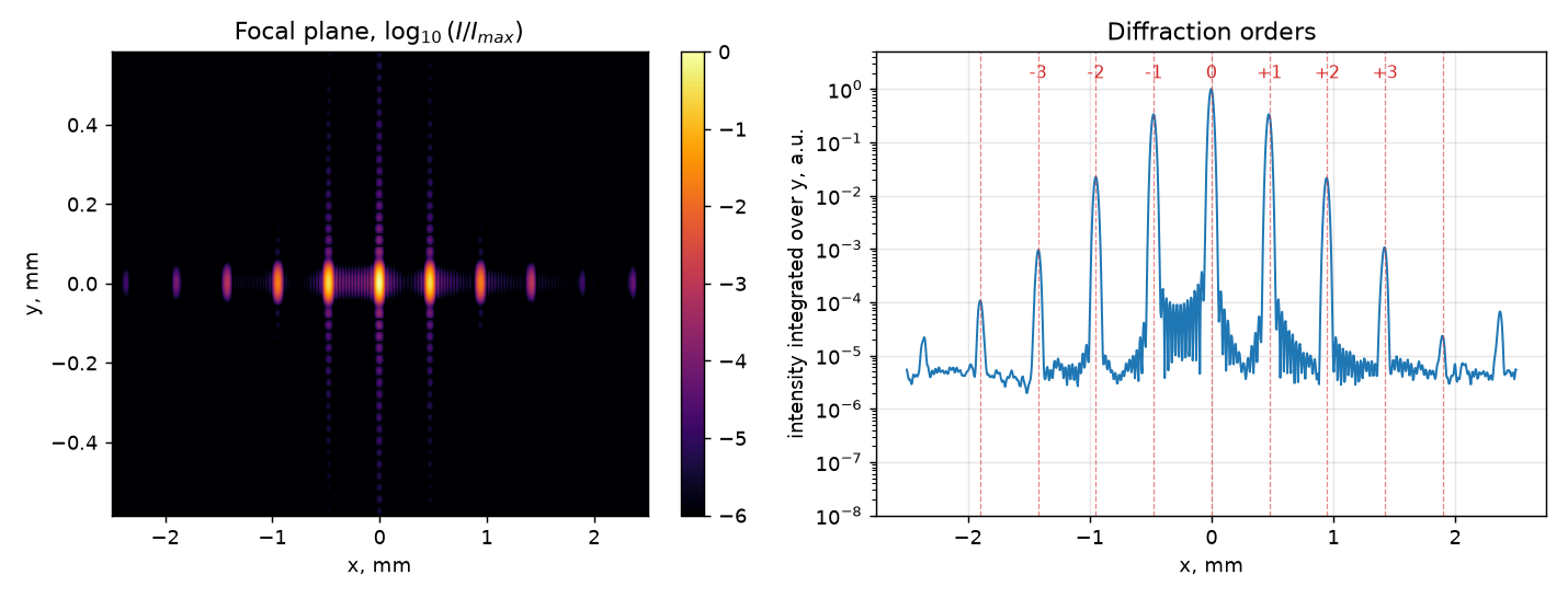

Focal plane

The five central spots are the $0, \pm 1, \pm 2$ orders, sitting exactly at the predicted positions (dashed lines). The horizontal fringes around each spot are the diffraction pattern of the square SLM aperture.

Step 3: Comparison with theory

Integrating the intensity inside a window of one order spacing around each peak gives the power in that order:


def order_powers(intensity, orders):
    Ix = intensity.sum(dim=0).numpy()
    out = []
    for n in orders:
        p = n * spacing
        sel = (x > p - spacing / 2) & (x < p + spacing / 2)
        out.append(Ix[sel].sum())
    return np.array(out) / Ix.sum()
 
def bessel_j(n, z, m=40001):
    """J_n(z) via the integral representation."""
    t = np.linspace(0, np.pi, m)
    return np.trapezoid(np.cos(n * t - z * np.sin(t)), t) / np.pi
 
orders = np.arange(-4, 5)
measured = order_powers(I, orders)
theory = np.array([bessel_j(n, DEPTH / 2) ** 2 for n in orders])

Order $n$	SVETlANNa	$J_n^2(m/2)$
0	0.5813	0.5855
±1	0.1954 / 0.1962	0.1936
±2	0.0131 / 0.0125	0.0132
±3	0.0006 / 0.0007	0.0004

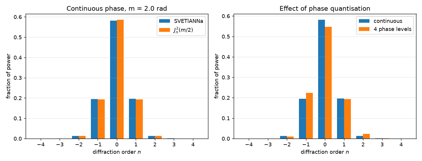
Order powers versus the Bessel prediction

The agreement is within a fraction of a percent; the residual comes from the finite aperture of the modulator, which is not part of the infinite-grating model.

Step 4: Phase quantisation

A real SLM applies a discrete set of phase levels. SpatialLightModulator models this through lut_function — a lookup table applied to the mask values. The helper QuantizerFromStepFunction turns any smooth one-step function into a differentiable quantiser, so a quantised SLM can still be trained end to end.


lut = sv.PartialWithParameters(
    QuantizerFromStepFunction(
        N=4,                       # 4 phase levels
        max_value=DEPTH,
        one_step_function=one_step_tanh,
    ),
    alpha=torch.tensor(30.0),      # steepness of the transition
)
 
slm_q = SpatialLightModulator(
    params, mask=mask, height=NPIX * PITCH, width=NPIX * PITCH, lut_function=lut,
)
setup_q = LinearOpticalSetup([
    slm_q,
    ThinLens(params, focal_length=F),
    FreeSpace(params, distance=F, method="zpRSC"),
])
 
measured_q = order_powers(setup_q(incident).intensity.detach(), orders)

With four levels the staircase is no longer symmetric, so power leaks asymmetrically into the neighbouring orders: the $-1$ order grows from 0.195 to 0.224 while the zero order drops from 0.581 to 0.548 (right-hand panel of the figure above).

alpha controls how sharp the steps are. Large values give a nearly ideal staircase but a vanishing gradient — start training with a small alpha and increase it gradually.

Full code


import math
import numpy as np
import torch
 
import svetlanna as sv
from svetlanna import SimulationParameters, Wavefront, LinearOpticalSetup
from svetlanna.elements import SpatialLightModulator, ThinLens, FreeSpace
from svetlanna.units import ureg
 
params = SimulationParameters.from_ranges(
    x_range=(-2.5 * ureg.mm, 2.5 * ureg.mm), x_points=1024,
    y_range=(-2.5 * ureg.mm, 2.5 * ureg.mm), y_points=1024,
    wavelength=632.8 * ureg.nm,
)
 
PITCH, NPIX = 8 * ureg.um, 400
PERIOD, DEPTH, F = 200 * ureg.um, 2.0, 150 * ureg.mm
 
px = (torch.arange(NPIX) - (NPIX - 1) / 2) * PITCH
mask_x, _ = torch.meshgrid(px, px, indexing="xy")
mask = (DEPTH / 2) * (1 + torch.sin(2 * math.pi * mask_x / PERIOD))
 
setup = LinearOpticalSetup([
    SpatialLightModulator(params, mask=mask,
                          height=NPIX * PITCH, width=NPIX * PITCH),
    ThinLens(params, focal_length=F),
    FreeSpace(params, distance=F, method="zpRSC"),
])
 
focal = setup(Wavefront.gaussian_beam(params, waist_radius=1.0 * ureg.mm))
 
x = params.x.numpy()
Ix = focal.intensity.detach().sum(dim=0).numpy()
spacing = float(632.8 * ureg.nm) * F / PERIOD
 
for n in range(-2, 3):
    sel = (x > n * spacing - spacing / 2) & (x < n * spacing + spacing / 2)
    print(f"order {n:+d}: {Ix[sel].sum() / Ix.sum():.4f}")

Things to try

Change DEPTH to $2.405 \cdot 2$ — the first zero of $J_0$ — and the zero order vanishes.
Replace the sinusoid with a sawtooth (torch.remainder) to obtain a blazed grating that sends almost all the power into a single order.
Rotate the grating by writing mask as a function of $x\cos\theta + y\sin\theta$ .
Wrap mask in torch.nn.Parameter and optimise it — every step above is differentiable.